pypercolate Tutorial
Bond percolation on linear chains and square lattices
This tutorial demonstrates how to use the pypercolate package. As examples, we present bond percolation with spanning cluster detection on a linear chain and a square grid of variable size, respectively.
Preamble
# configure plotting
%config InlineBackend.rc = {'figure.dpi': 300, 'savefig.dpi': 300, \
                            'figure.figsize': (10, 5), 'font.size': 12, \
                            'figure.facecolor': (1, 1, 1, 0)}
%matplotlib inline

# import packages
import numpy as np
import matplotlib as mpl
import matplotlib.pyplot as plt
import networkx as nx
import percolate
from pprint import pprint

# configure plotting colors
colors = [
    '#0e5a94',
    '#eb008a',
    '#37b349',
    '#f29333',
    '#00aabb',
    '#b31e8d',
    '#f8ca12',
    '#7a2d00',
]
mpl.rcParams['axes.color_cycle'] = colors
Evolution of one sample state (realization)
First, we get to know the basic unit of computation in the Newman-Ziff
algorithm: a single sample state (realization). The sample_states
generator function evolves a single realization by successively adding
bonds, incrementing the occupation number \(n\) by \(1\) in each
step.
Linear chain
# Generate linear chain graph with auxiliary nodes for spanning cluster detection
chain = percolate.spanning_1d_chain(length=10)
# Evolve sample state and plot it at the same time
edges = list()
fig, axes = plt.subplots(figsize=(8.0, 2.0), ncols=5, nrows=2, squeeze=True)
axes = axes.ravel()
for i, sample_state in enumerate(percolate.sample_states(chain)):
    if 'edge' in sample_state:
        edge = sample_state['edge']
        edges.append(edge)
    nx.draw(
        chain,
        ax=axes[i],
        edgelist=edges,
        width=4,
        pos={node: (node, 0) for node in chain.nodes_iter()},
        node_size=10,
    )
    axes[i].set_title('n = {}'.format(i))
    pprint(sample_state)
plt.tight_layout(0)
plt.show()
{'M': 9,
 'N': 10,
 'has_spanning_cluster': False,
 'max_cluster_size': 1,
 'moments': array([ 9.,  9.,  9.,  9.,  9.]),
 'n': 0}
{'M': 9,
 'N': 10,
 'edge': (6, 7),
 'has_spanning_cluster': False,
 'max_cluster_size': 2,
 'moments': array([ 8.,  8.,  8.,  8.,  8.]),
 'n': 1}
{'M': 9,
 'N': 10,
 'edge': (3, 4),
 'has_spanning_cluster': False,
 'max_cluster_size': 2,
 'moments': array([  7.,   8.,  10.,  14.,  22.]),
 'n': 2}
{'M': 9,
 'N': 10,
 'edge': (7, 8),
 'has_spanning_cluster': False,
 'max_cluster_size': 3,
 'moments': array([  6.,   7.,   9.,  13.,  21.]),
 'n': 3}
{'M': 9,
 'N': 10,
 'edge': (5, 6),
 'has_spanning_cluster': False,
 'max_cluster_size': 4,
 'moments': array([  5.,   6.,   8.,  12.,  20.]),
 'n': 4}
{'M': 9,
 'N': 10,
 'edge': (9, 10),
 'has_spanning_cluster': False,
 'max_cluster_size': 4,
 'moments': array([  4.,   6.,  10.,  18.,  34.]),
 'n': 5}
{'M': 9,
 'N': 10,
 'edge': (8, 9),
 'has_spanning_cluster': False,
 'max_cluster_size': 6,
 'moments': array([  3.,   4.,   6.,  10.,  18.]),
 'n': 6}
{'M': 9,
 'N': 10,
 'edge': (1, 2),
 'has_spanning_cluster': False,
 'max_cluster_size': 6,
 'moments': array([  2.,   4.,   8.,  16.,  32.]),
 'n': 7}
{'M': 9,
 'N': 10,
 'edge': (2, 3),
 'has_spanning_cluster': False,
 'max_cluster_size': 6,
 'moments': array([   1.,    4.,   16.,   64.,  256.]),
 'n': 8}
{'M': 9,
 'N': 10,
 'edge': (4, 5),
 'has_spanning_cluster': True,
 'max_cluster_size': 10,
 'moments': array([ 0.,  0.,  0.,  0.,  0.]),
 'n': 9}
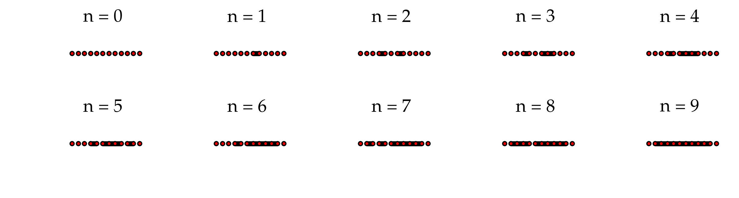
Figure: Evolution of a single realization of bond percolation on the linear chain with 10 nodes. The terminal nodes are the auxiliary nodes for spanning cluster detection.
Square grid
# Generate square grid graph with auxiliary nodes for spanning cluster detection
grid = percolate.spanning_2d_grid(3)
# Evolve sample state and plot it at the same time
edges = list()
fig, axes = plt.subplots(figsize=(8.0, 4.0), ncols=4, nrows=3, squeeze=True)
axes = axes.ravel()
for i, sample_state in enumerate(percolate.sample_states(grid)):
    if 'edge' in sample_state:
        edge = sample_state['edge']
        edges.append(edge)
        nx.draw(
            grid,
            ax=axes[i - 1],
            edgelist=edges,
            width=4,
            pos={node: node for node in grid.nodes_iter()},
            node_size=100,
        )
        axes[i - 1].set_title('n = {}'.format(i))
    pprint(sample_state)
plt.tight_layout(0)
plt.show()
{'M': 12,
 'N': 9,
 'has_spanning_cluster': False,
 'max_cluster_size': 1,
 'moments': array([ 8.,  8.,  8.,  8.,  8.]),
 'n': 0}
{'M': 12,
 'N': 9,
 'edge': ((2, 0), (3, 0)),
 'has_spanning_cluster': False,
 'max_cluster_size': 2,
 'moments': array([ 7.,  7.,  7.,  7.,  7.]),
 'n': 1}
{'M': 12,
 'N': 9,
 'edge': ((1, 2), (1, 1)),
 'has_spanning_cluster': False,
 'max_cluster_size': 2,
 'moments': array([  6.,   7.,   9.,  13.,  21.]),
 'n': 2}
{'M': 12,
 'N': 9,
 'edge': ((3, 2), (3, 1)),
 'has_spanning_cluster': False,
 'max_cluster_size': 2,
 'moments': array([  5.,   7.,  11.,  19.,  35.]),
 'n': 3}
{'M': 12,
 'N': 9,
 'edge': ((2, 0), (1, 0)),
 'has_spanning_cluster': True,
 'max_cluster_size': 3,
 'moments': array([  4.,   6.,  10.,  18.,  34.]),
 'n': 4}
{'M': 12,
 'N': 9,
 'edge': ((1, 2), (2, 2)),
 'has_spanning_cluster': True,
 'max_cluster_size': 3,
 'moments': array([  3.,   6.,  14.,  36.,  98.]),
 'n': 5}
{'M': 12,
 'N': 9,
 'edge': ((3, 0), (3, 1)),
 'has_spanning_cluster': True,
 'max_cluster_size': 5,
 'moments': array([  2.,   4.,  10.,  28.,  82.]),
 'n': 6}
{'M': 12,
 'N': 9,
 'edge': ((2, 2), (2, 1)),
 'has_spanning_cluster': True,
 'max_cluster_size': 5,
 'moments': array([   1.,    4.,   16.,   64.,  256.]),
 'n': 7}
{'M': 12,
 'N': 9,
 'edge': ((3, 2), (2, 2)),
 'has_spanning_cluster': True,
 'max_cluster_size': 9,
 'moments': array([ 0.,  0.,  0.,  0.,  0.]),
 'n': 8}
{'M': 12,
 'N': 9,
 'edge': ((3, 1), (2, 1)),
 'has_spanning_cluster': True,
 'max_cluster_size': 9,
 'moments': array([ 0.,  0.,  0.,  0.,  0.]),
 'n': 9}
{'M': 12,
 'N': 9,
 'edge': ((1, 1), (2, 1)),
 'has_spanning_cluster': True,
 'max_cluster_size': 9,
 'moments': array([ 0.,  0.,  0.,  0.,  0.]),
 'n': 10}
{'M': 12,
 'N': 9,
 'edge': ((2, 0), (2, 1)),
 'has_spanning_cluster': True,
 'max_cluster_size': 9,
 'moments': array([ 0.,  0.,  0.,  0.,  0.]),
 'n': 11}
{'M': 12,
 'N': 9,
 'edge': ((1, 0), (1, 1)),
 'has_spanning_cluster': True,
 'max_cluster_size': 9,
 'moments': array([ 0.,  0.,  0.,  0.,  0.]),
 'n': 12}
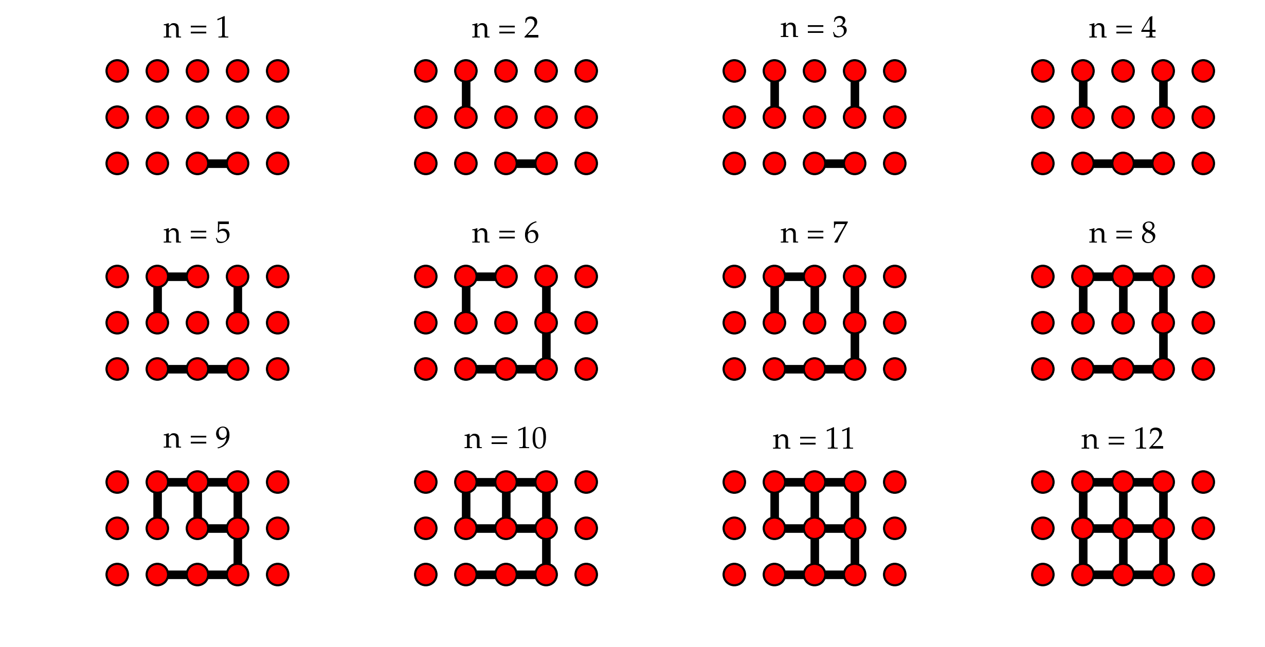
Figure: Evolution of a single realization of bond percolation on the 3x3 square grid. The left-hand and right-hand outermost nodes are the auxiliary nodes for spanning cluster detection.
Single run statistics
Now, we want to compare cluster statistics for several sample states (realizations) evolved in parallel. We also want to compare these statistics for several system sizes \(L\).
# number of parallel runs (sample states to evolve)
runs = 4
Linear chain
# system sizes
chain_ls = [10, 100, 1000, 10000]
# generate the linear chain graphs with spanning cluster detection
# for all system sizes
chain_graphs = [ percolate.spanning_1d_chain(l) for l in chain_ls ]
# compute the single-run cluster statistics for all sample states
# and system sizes
chain_single_runs = [
    [ percolate.single_run_arrays(graph=chain_graph) for _ in range(runs) ]
    for chain_graph in chain_graphs
]
# plot
fig, axes = plt.subplots(
    nrows=len(chain_ls), ncols=5, squeeze=True, figsize=(8.0, 6.0)
)
for l_index, l in enumerate(chain_ls):
    for single_run in chain_single_runs[l_index]:
        axes[l_index, 0].plot(
            single_run['has_spanning_cluster'], lw=4, alpha=0.7, rasterized=True
        )
        axes[l_index, 1].plot(
            single_run['max_cluster_size'], lw=4, alpha=0.7, rasterized=True
        )
        for k in range(3):
            axes[l_index, k + 2].plot(
                single_run['moments'][k], lw=4, alpha=0.7, rasterized=True
            )

    axes[l_index, 0].set_ylabel(r'L={}'.format(l))

    for ax in axes[l_index, :]:
        num_edges = chain_single_runs[l_index][0]['M']
        ax.set_xlim(xmax=1.05 * num_edges)
        ax.set_xticks([0, l / 2, l - 1])
        ax.set_yticks(np.linspace(0, ax.get_ylim()[1], num=3))

    axes[l_index, 0].set_yticks([0, 1])

axes[0, 0].set_title(r'spanning?')
axes[0, 1].set_title(r'largest cluster')
for k in range(3):
    axes[0, k + 2].set_title(r'$M_{}$'.format(k))

for ax in axes[-1, :]:
    ax.set_xlabel(r'$n$')

plt.tight_layout(0)
plt.show()
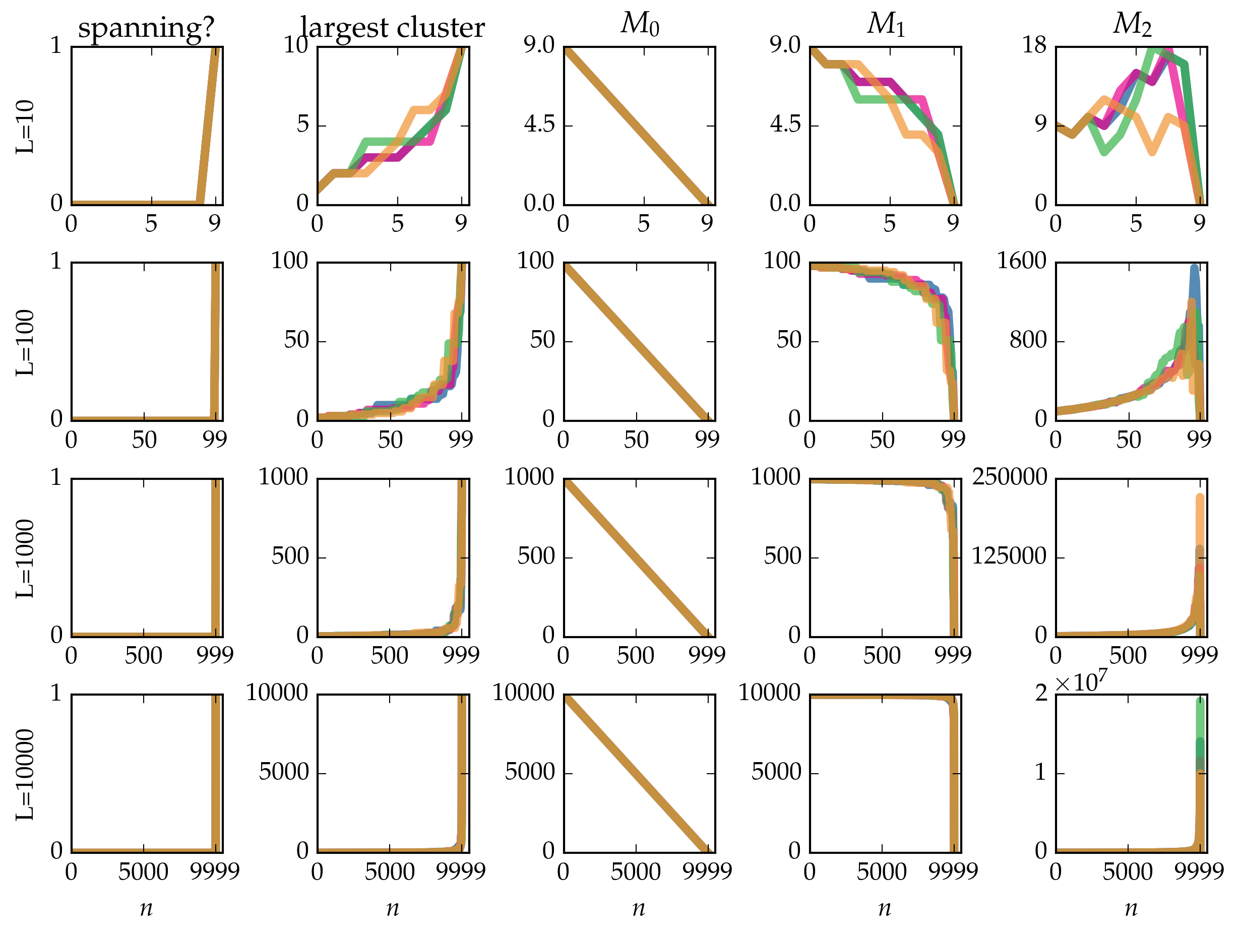
Figure: Cluster statistics for single realizations of bond percolation on the linear chain with \(L\) nodes, evolved according to the Newman-Ziff algorithm over all occupation numbers \(n = 0 \ldots L - 1\).
# clear memory
del chain_single_runs
Square grid
# system sizes
grid_ls = [3, 10, 32, 100, 316]
# generate the square grid graphs with spanning cluster detection
# for all system sizes
grid_graphs = [ percolate.spanning_2d_grid(l) for l in grid_ls ]
# compute the single-run cluster statistics for all sample states
# and system sizes
grid_single_runs = [
    [ percolate.single_run_arrays(graph=grid_graph) for _ in range(runs) ]
    for grid_graph in grid_graphs
]
# plot
fig, axes = plt.subplots(
    nrows=len(grid_ls), ncols=5, squeeze=True, figsize=(8.0, 6.0)
)
for l_index, l in enumerate(grid_ls):
    for single_run in grid_single_runs[l_index]:
        axes[l_index, 0].plot(
            single_run['has_spanning_cluster'], lw=4, alpha=0.7, rasterized=True
        )
        axes[l_index, 1].plot(
            single_run['max_cluster_size'], lw=4, alpha=0.7, rasterized=True
        )
        for k in range(3):
            axes[l_index, k + 2].plot(
                single_run['moments'][k], lw=4, alpha=0.7, rasterized=True
            )

    axes[l_index, 0].set_ylabel(r'L={}'.format(l))

    for ax in axes[l_index, :]:
        num_edges = grid_single_runs[l_index][0]['M']
        ax.set_xlim(xmax=num_edges)
        ax.set_xticks(np.linspace(0, num_edges, num=3))
        ax.set_xticklabels(['0', '', num_edges])
        ax.set_yticks(np.linspace(0, ax.get_ylim()[1], num=3))

    axes[l_index, 0].set_yticks([0, 1])

axes[0, 0].set_title(r'spanning?')
axes[0, 1].set_title(r'largest cluster')
for k in range(3):
    axes[0, k + 2].set_title(r'$M_{}$'.format(k))

for ax in axes[-1, :]:
    ax.set_xlabel(r'$n$')

plt.tight_layout(0)
plt.show()
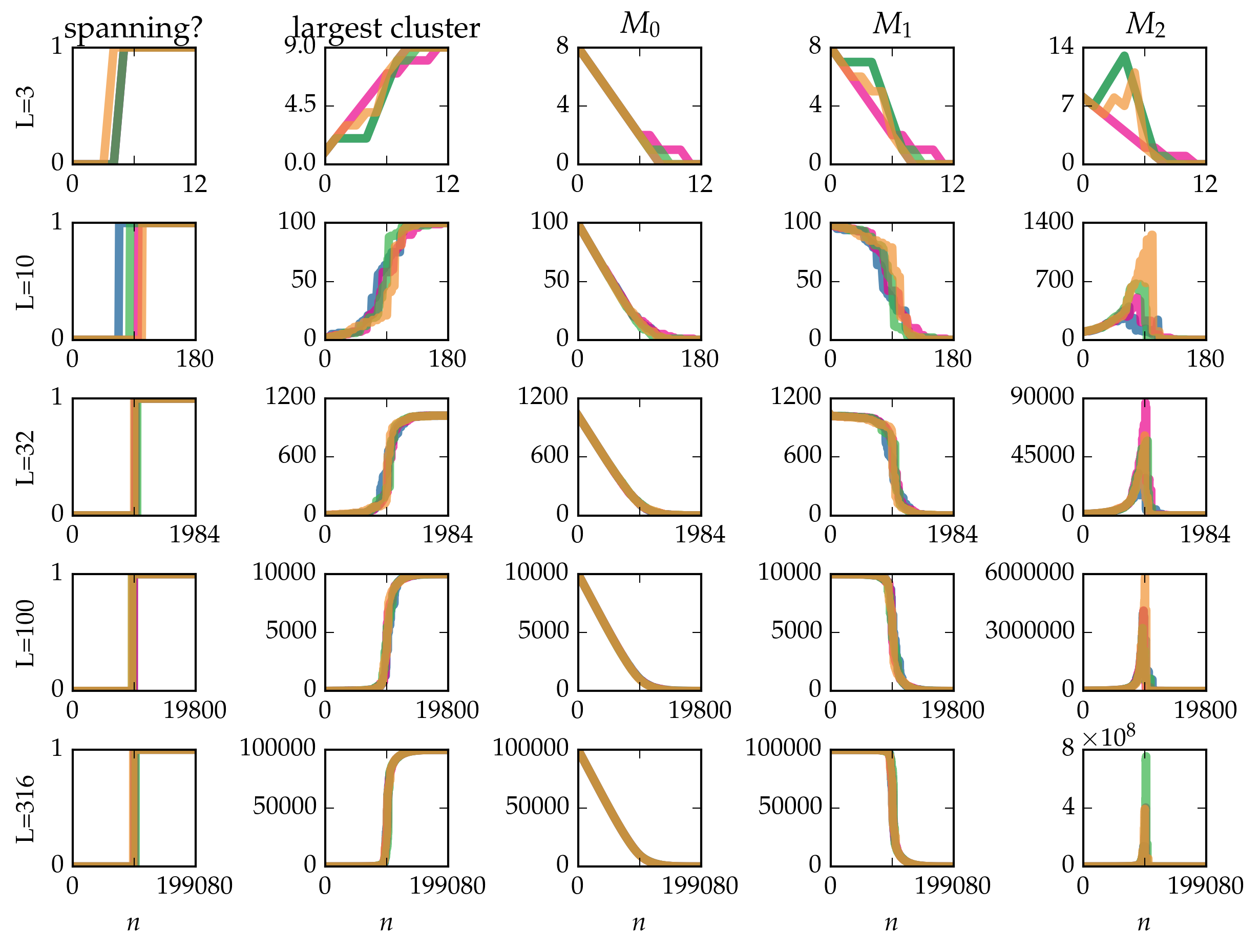
Figure: Cluster statistics for single realizations of bond percolation on the \(L \times L\) square grid, evolved according to the Newman-Ziff algorithm over all occupation numbers \(n = 0 \ldots 2 L (L - 1)\).
# clear memory
del grid_single_runs
Microcanonical ensemble averages
Next we explore how pypercolate enables us to aggregate cluster statistics across a number of runs (realizations), evolved over all occupation numbers. For each occupation number, this yields the microcanonical average.
Linear chain
# number of runs
chain_runs = 40
# system sizes
chain_ls = [10, 100, 1000, 10000]
# generate the linear chain graphs with spanning cluster detection
# for all system sizes
chain_graphs = [ percolate.spanning_1d_chain(l) for l in chain_ls ]
# compute the microcanonical averages for all system sizes
chain_microcanonical_averages = [
    percolate.microcanonical_averages(
        graph=chain_graph, runs=chain_runs
    )
    for chain_graph in chain_graphs
]
# combine microcanonical averages into one array
chain_microcanonical_averages_arrays = [
    percolate.microcanonical_averages_arrays(avg)
    for avg in chain_microcanonical_averages
]
# plot
fig, axes = plt.subplots(
    nrows=len(chain_ls), ncols=3, squeeze=True, figsize=(8.0, 6.0)
)
for l_index, l in enumerate(chain_ls):
    avg_arrays = chain_microcanonical_averages_arrays[l_index]

    line, = axes[l_index, 0].plot(
        np.arange(avg_arrays['M'] + 1),
        avg_arrays['spanning_cluster'],
        rasterized=True,
    )
    axes[l_index, 0].fill_between(
        np.arange(avg_arrays['M'] + 1),
        avg_arrays['spanning_cluster_ci'].T[1],
        avg_arrays['spanning_cluster_ci'].T[0],
        facecolor=line.get_color(),
        alpha=0.5,
        rasterized=True,
    )

    line, = axes[l_index, 1].plot(
        np.arange(avg_arrays['M'] + 1),
        avg_arrays['max_cluster_size'],
        rasterized=True,
    )
    axes[l_index, 1].fill_between(
        np.arange(avg_arrays['M'] + 1),
        avg_arrays['max_cluster_size_ci'].T[1],
        avg_arrays['max_cluster_size_ci'].T[0],
        facecolor=line.get_color(),
        alpha=0.5,
        rasterized=True,
    )

    axes[l_index, 2].plot(
        np.arange(avg_arrays['M'] + 1),
        avg_arrays['moments'][2],
        rasterized=True,
    )
    axes[l_index, 2].fill_between(
        np.arange(avg_arrays['M'] + 1),
        avg_arrays['moments_ci'][2].T[1],
        avg_arrays['moments_ci'][2].T[0],
        facecolor=line.get_color(),
        alpha=0.5,
        rasterized=True,
    )


    axes[l_index, 0].set_ylabel(r'L={}'.format(l))
    axes[l_index, 1].set_ylim(ymax=1.0)
    axes[l_index, 2].set_ylim(ymin=0.0)

    for ax in axes[l_index, :]:
        num_edges = avg_arrays['M']
        ax.set_xlim(xmax=1.05 * num_edges)
        ax.set_xticks([0, l / 2, num_edges])
        ax.set_yticks(np.linspace(0, ax.get_ylim()[1], num=3))

axes[0, 0].set_title(r'percolation probability')
axes[0, 1].set_title(r'percolation strength')
axes[0, 2].set_title(r'$\langle M_2 \rangle$')

for ax in axes[-1, :]:
    ax.set_xlabel(r'$n$')

plt.tight_layout(0)
plt.show()
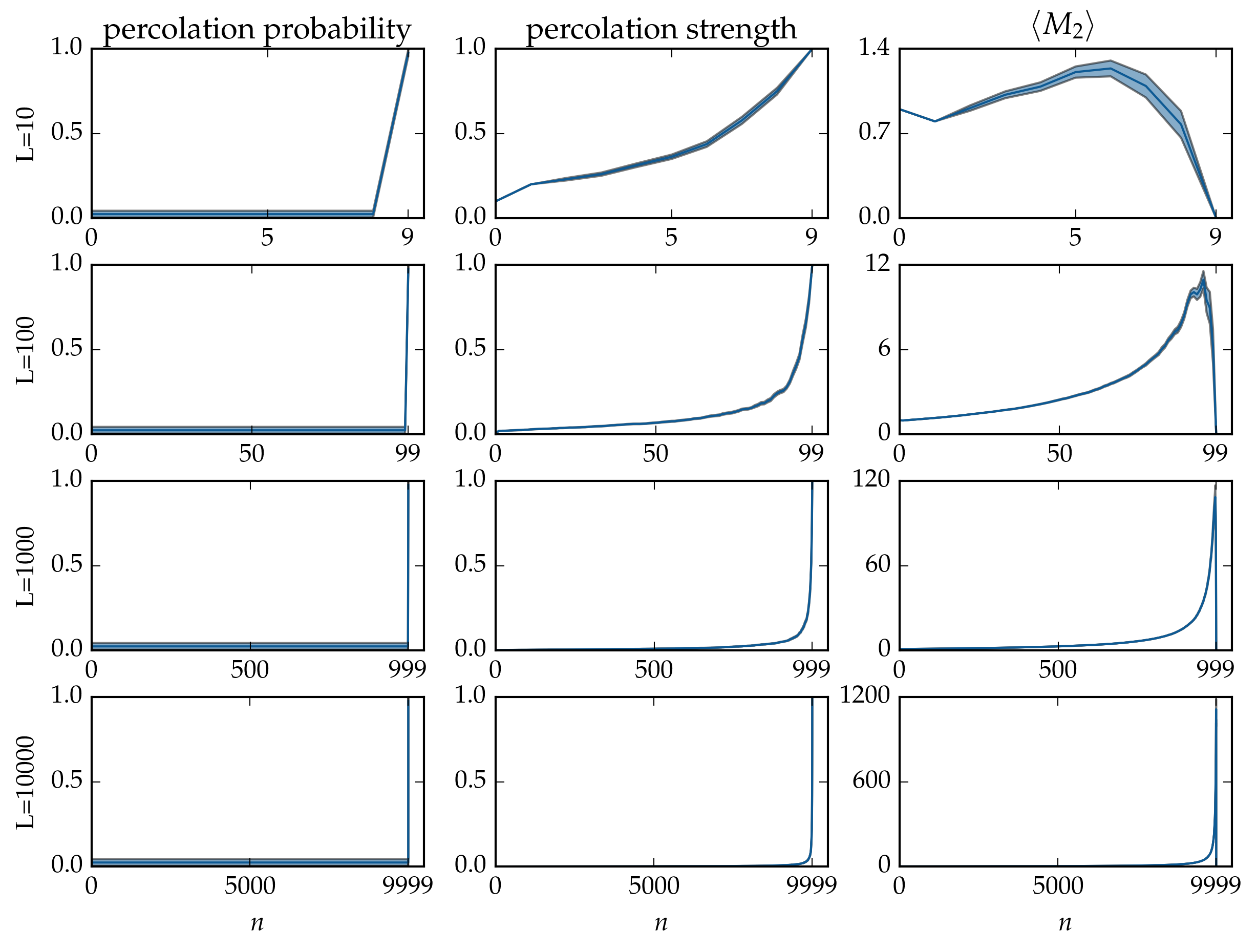
Figure: Microcanonical averages of cluster statistics of bond percolation on the linear chain with \(L\) nodes, over \(40\) runs. The samples of the microcanonical ensembles have been evolved by the Newman-Ziff algorithm over all occupation numbers \(n = 0 \ldots L - 1\).
Square grid
# number of runs
grid_runs = 40
# system sizes
grid_ls = [3, 10, 32, 100, 316]
# generate the square grid graphs with spanning cluster detection
# for all system sizes
grid_graphs = [ percolate.spanning_2d_grid(l) for l in grid_ls ]
# compute the microcanonical averages for all system sizes
grid_microcanonical_averages = [
    percolate.microcanonical_averages(
        graph=grid_graph, runs=grid_runs
    )
    for grid_graph in grid_graphs
]
# combine microcanonical averages into one array
grid_microcanonical_averages_arrays = [
    percolate.microcanonical_averages_arrays(avg)
    for avg in grid_microcanonical_averages
]
# plot
fig, axes = plt.subplots(
    nrows=len(grid_ls), ncols=3, squeeze=True, figsize=(8.0, 6.0)
)
for l_index, l in enumerate(grid_ls):
    avg_arrays = grid_microcanonical_averages_arrays[l_index]

    line, = axes[l_index, 0].plot(
        np.arange(avg_arrays['M'] + 1),
        avg_arrays['spanning_cluster'],
        rasterized=True,
    )
    axes[l_index, 0].fill_between(
        np.arange(avg_arrays['M'] + 1),
        avg_arrays['spanning_cluster_ci'].T[1],
        avg_arrays['spanning_cluster_ci'].T[0],
        facecolor=line.get_color(),
        alpha=0.5,
        rasterized=True,
    )

    line, = axes[l_index, 1].plot(
        np.arange(avg_arrays['M'] + 1),
        avg_arrays['max_cluster_size'],
        rasterized=True,
    )
    axes[l_index, 1].fill_between(
        np.arange(avg_arrays['M'] + 1),
        avg_arrays['max_cluster_size_ci'].T[1],
        avg_arrays['max_cluster_size_ci'].T[0],
        facecolor=line.get_color(),
        alpha=0.5,
        rasterized=True,
    )

    axes[l_index, 2].plot(
        np.arange(avg_arrays['M'] + 1),
        avg_arrays['moments'][2],
        rasterized=True,
    )
    axes[l_index, 2].fill_between(
        np.arange(avg_arrays['M'] + 1),
        avg_arrays['moments_ci'][2].T[1],
        avg_arrays['moments_ci'][2].T[0],
        facecolor=line.get_color(),
        alpha=0.5,
        rasterized=True,
    )


    axes[l_index, 0].set_ylabel(r'L={}'.format(l))
    axes[l_index, 1].set_ylim(ymax=1.0)
    axes[l_index, 2].set_ylim(ymin=0.0)

    for ax in axes[l_index, :]:
        num_edges = avg_arrays['M']
        ax.set_xlim(xmax=num_edges)
        ax.set_xticks(np.linspace(0, num_edges, num=3))
        ax.set_yticks(np.linspace(0, ax.get_ylim()[1], num=3))

axes[0, 0].set_title(r'percolation probability')
axes[0, 1].set_title(r'percolation strength')
axes[0, 2].set_title(r'$\langle M_2 \rangle$')

for ax in axes[-1, :]:
    ax.set_xlabel(r'$n$')

plt.tight_layout(0)
plt.show()
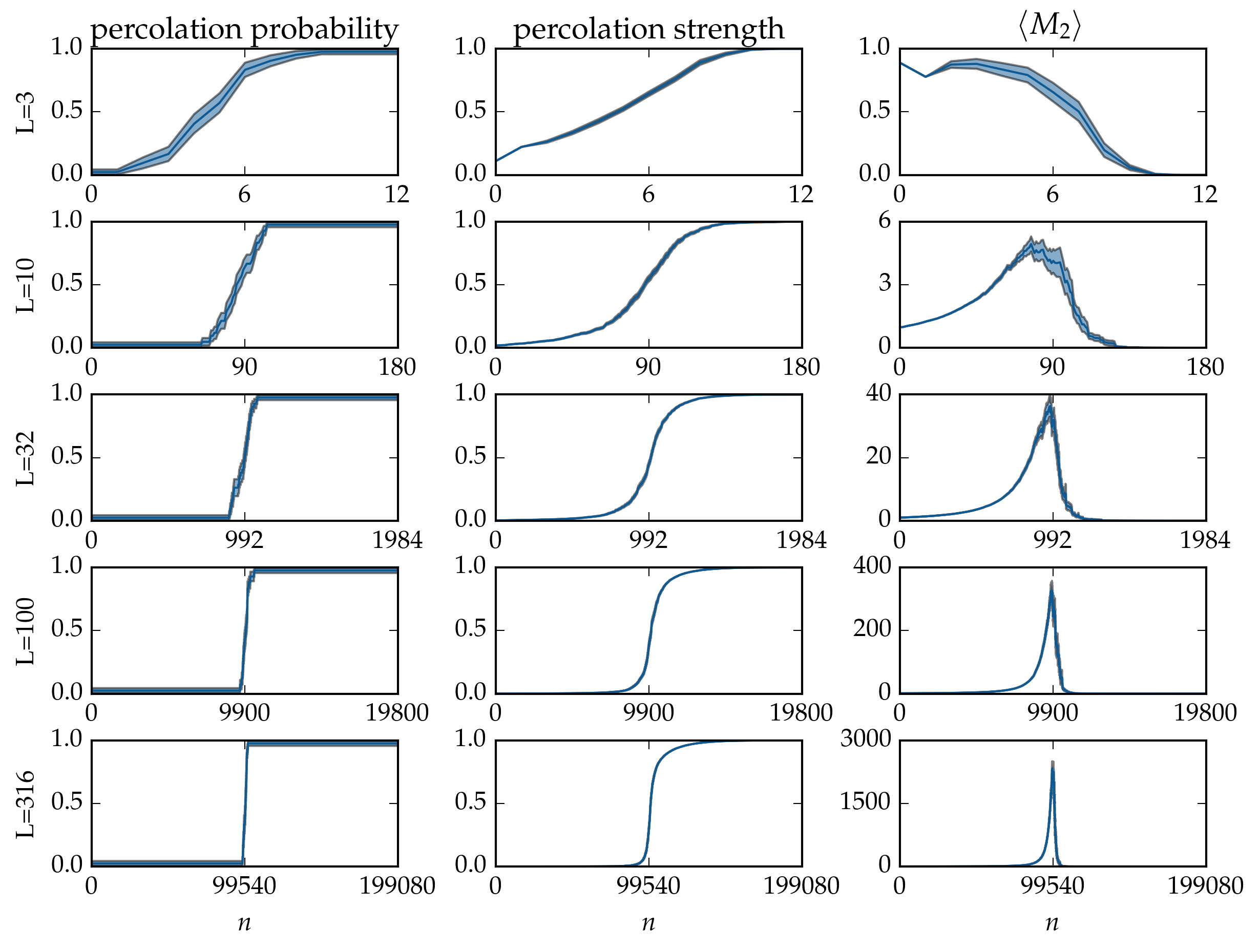
Figure: Microcanonical averages of cluster statistics of bond percolation on the \(L \times L\) square grid, over \(40\) runs. The samples of the microcanonical ensembles have been evolved by the Newman-Ziff algorithm over all occupation numbers \(n = 0 \ldots 2 L (L - 1)\).
Canonical ensemble averages
Having computed the microcanonical averages for all occupation numbers \(n\), the last step is to transform them to canonical averages for the desired values of the occupation probability \(p\).
Linear chain
# occupation probabilities
chain_ps_arrays = [ np.linspace(1.0 - x, 1.0, num=100) for x in [1.0, 0.1, 0.01] ]
# compute canonical averages from microcanonical averages
# for all occupation probabilities and system sizes
chain_stats = [
    [
        percolate.canonical_averages(ps, avg_arrays)
        for avg_arrays in chain_microcanonical_averages_arrays
    ]
    for ps in chain_ps_arrays
]
# plot
fig, axes = plt.subplots(
    nrows=len(chain_ps_arrays), ncols=4, squeeze=True, figsize=(8.0, 4.5)
)
for ps_index, ps in enumerate(chain_ps_arrays):
    for l_index, l in enumerate(chain_ls):
        my_stats = chain_stats[ps_index][l_index]

        line, = axes[ps_index, 0].plot(
            ps,
            my_stats['spanning_cluster'],
            rasterized=True,
            label=r'{}'.format(l),
        )
        axes[ps_index, 0].fill_between(
            ps,
            my_stats['spanning_cluster_ci'].T[1],
            my_stats['spanning_cluster_ci'].T[0],
            facecolor=line.get_color(),
            alpha=0.5,
            rasterized=True,
        )

        line, = axes[ps_index, 1].plot(
            ps,
            my_stats['max_cluster_size'],
            rasterized=True,
            label=r'L={}'.format(l),
        )
        axes[ps_index, 1].fill_between(
            ps,
            my_stats['max_cluster_size_ci'].T[1],
            my_stats['max_cluster_size_ci'].T[0],
            facecolor=line.get_color(),
            alpha=0.5,
            rasterized=True,
        )

        axes[ps_index, 2].plot(
            ps,
            my_stats['moments'][2],
            rasterized=True,
            label=r'L={}'.format(l),
        )
        axes[ps_index, 2].fill_between(
            ps,
            my_stats['moments_ci'][2].T[1],
            my_stats['moments_ci'][2].T[0],
            facecolor=line.get_color(),
            alpha=0.5,
            rasterized=True,
        )

        axes[ps_index, 3].semilogy(
            ps,
            my_stats['moments'][2],
            rasterized=True,
        )
        axes[ps_index, 3].fill_between(
            ps,
            np.where(
                my_stats['moments_ci'][2].T[1] > 0.0,
                my_stats['moments_ci'][2].T[1],
                0.01
            ),
            np.where(
                my_stats['moments_ci'][2].T[0] > 0.0,
                my_stats['moments_ci'][2].T[0],
                0.01
            ),
            facecolor=line.get_color(),
            alpha=0.5,
            rasterized=True,
        )


    axes[ps_index, 0].set_ylim(ymax=1.0)
    axes[ps_index, 1].set_ylim(ymax=1.0)
    axes[ps_index, 2].set_ylim(ymin=0.0)
    axes[ps_index, 3].set_ylim(ymin=0.5)

    for ax in axes[ps_index, :]:
        ax.set_xlim(xmin=ps.min(), xmax=ps.max() + (ps.max() - ps.min()) * 0.05)
        ax.set_xticks(np.linspace(ps.min(), ps.max(), num=3))

    for ax in axes[ps_index, :-1]:
        ax.set_yticks(np.linspace(0, ax.get_ylim()[1], num=3))

axes[0, 0].set_title(r'perc. probability')
axes[0, 1].set_title(r'perc. strength')
axes[0, 2].set_title(r'$\langle M_2 \rangle$')
axes[0, 3].set_title(r'$\langle M_2 \rangle$')

for ax in axes[-1, :]:
    ax.set_xlabel(r'$p$')

axes[0, 2].legend(frameon=False, loc='center left')

plt.tight_layout(0)
plt.show()
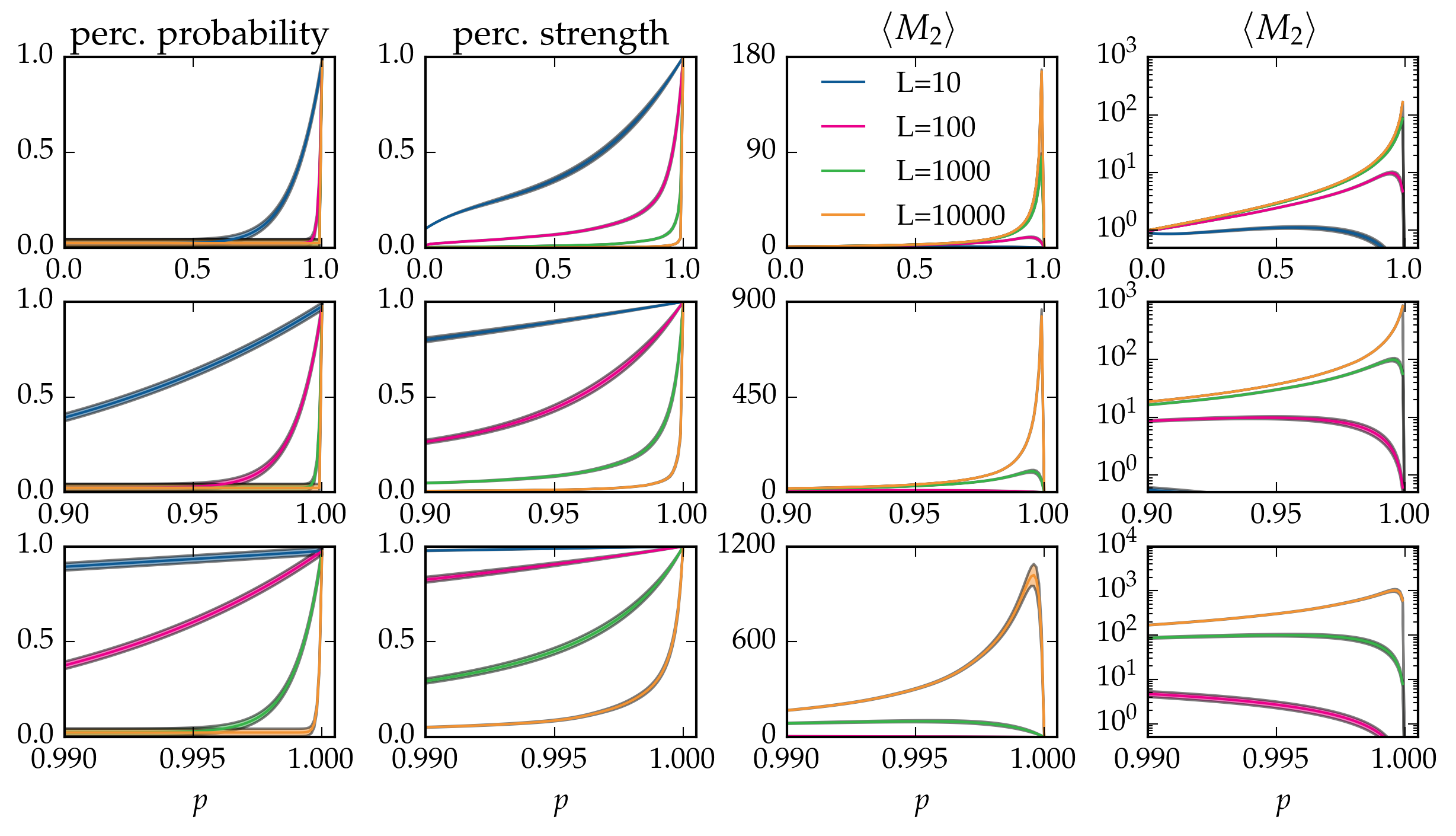
Figure: Canonical averages of cluster statistics of bond percolation on the linear chain with \(L\) nodes, over \(40\) runs.
Square grid
# occupation probabilities
grid_ps_arrays = [ np.linspace(0.5 - x, 0.5 + x, num=100) for x in [0.5, 0.05] ]
# compute canonical averages from microcanonical averages
# for all occupation probabilities and system sizes
grid_stats = [
    [
        percolate.canonical_averages(ps, avg_arrays)
        for avg_arrays in grid_microcanonical_averages_arrays
    ]
    for ps in grid_ps_arrays
]
# plot
fig, axes = plt.subplots(
    nrows=len(grid_ps_arrays), ncols=4, squeeze=True, figsize=(8.0, 4.5)
)
for ps_index, ps in enumerate(grid_ps_arrays):
    for l_index, l in enumerate(grid_ls):
        my_stats = grid_stats[ps_index][l_index]

        line, = axes[ps_index, 0].plot(
            ps,
            my_stats['spanning_cluster'],
            rasterized=True,
            label=r'L={}'.format(l),
        )
        axes[ps_index, 0].fill_between(
            ps,
            my_stats['spanning_cluster_ci'].T[1],
            my_stats['spanning_cluster_ci'].T[0],
            facecolor=line.get_color(),
            alpha=0.5,
            rasterized=True,
        )

        line, = axes[ps_index, 1].plot(
            ps,
            my_stats['max_cluster_size'],
            rasterized=True,
            label=r'L={}'.format(l),
        )
        axes[ps_index, 1].fill_between(
            ps,
            my_stats['max_cluster_size_ci'].T[1],
            my_stats['max_cluster_size_ci'].T[0],
            facecolor=line.get_color(),
            alpha=0.5,
            rasterized=True,
        )

        axes[ps_index, 2].plot(
            ps,
            my_stats['moments'][2],
            rasterized=True,
            label=r'L={}'.format(l),
        )
        axes[ps_index, 2].fill_between(
            ps,
            my_stats['moments_ci'][2].T[1],
            my_stats['moments_ci'][2].T[0],
            facecolor=line.get_color(),
            alpha=0.5,
            rasterized=True,
        )

        axes[ps_index, 3].semilogy(
            ps,
            my_stats['moments'][2],
            rasterized=True,
        )
        axes[ps_index, 3].fill_between(
            ps,
            np.where(
                my_stats['moments_ci'][2].T[1] > 0.0,
                my_stats['moments_ci'][2].T[1],
                0.01
            ),
            np.where(
                my_stats['moments_ci'][2].T[0] > 0.0,
                my_stats['moments_ci'][2].T[0],
                0.01
            ),
            facecolor=line.get_color(),
            alpha=0.5,
            rasterized=True,
        )


    axes[ps_index, 0].set_ylim(ymax=1.0)
    axes[ps_index, 1].set_ylim(ymax=1.0)
    axes[ps_index, 2].set_ylim(ymin=0.0)
    axes[ps_index, 3].set_ylim(ymin=0.5)

    for ax in axes[ps_index, :]:
        ax.set_xlim(xmin=ps.min(), xmax=ps.max())
        ax.set_xticks(np.linspace(ps.min(), ps.max(), num=3))

    for ax in axes[ps_index, :-1]:
        ax.set_yticks(np.linspace(0, ax.get_ylim()[1], num=3))

axes[0, 0].set_title(r'perc. probability')
axes[0, 1].set_title(r'perc. strength')
axes[0, 2].set_title(r'$\langle M_2 \rangle$')
axes[0, 3].set_title(r'$\langle M_2 \rangle$')

for ax in axes[-1, :]:
    ax.set_xlabel(r'$p$')

axes[0, 2].legend(frameon=False, loc='best')

plt.tight_layout(0)
plt.show()
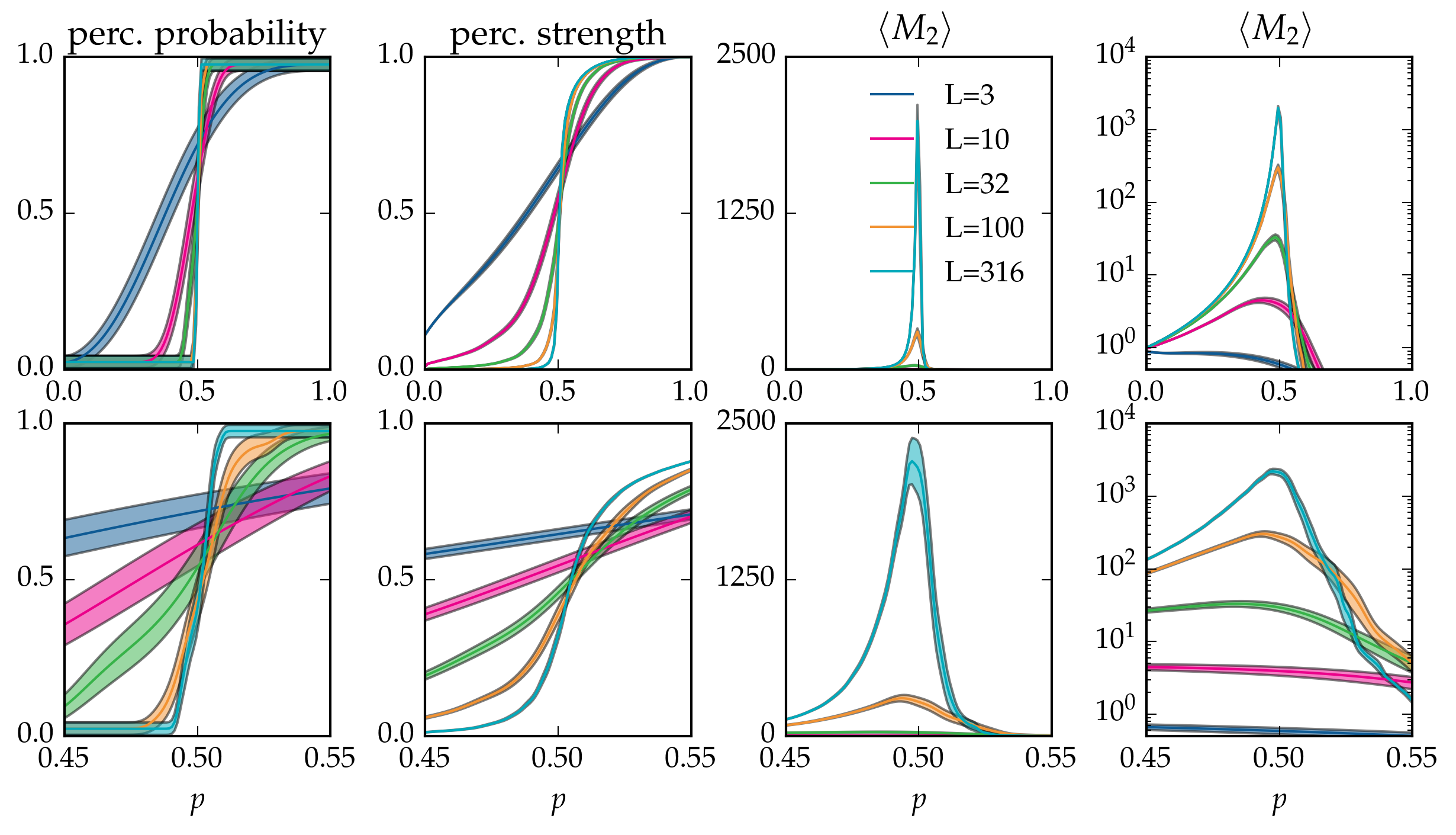
Figure: Canonical averages of cluster statistics of bond percolation on the \(L \times L\) square grid, over \(40\) runs.
